REVISTA MEXICANA DE CIENCIAS GEOLÓGICAS

DOI: http://dx.doi.org/10.22201/cgeo.20072902e.2021.3.1641

 

INTRODUCTION

Orientation data of rock strata and their discontinuities constitute a key knowledge element to characterize rock masses, which is crucial for many geoscientific and engineering applications. In structural geology, for instance, statistical analysis of orientation data allows reconstructing the history and evolution of an acting stress field (Ramsay and Huber, 1987; Davis et. al., 2011; Allmendinger, et al. 2011). In exploration geology, rock lineaments provide insights into different geometric patterns of ore deposits, oil/gas reservoirs, and fractured aquifers (Lerche, 1997; Fetter, 2001). In geotechnical engineering, dip and dip direction records are key inputs for developing slope-rock stability studies (Goodman, 1989; Hudson and Harrison, 1997).

To obtain rock strata and their discontinuities’ orientation datasets, the common practice requires a qualified professional to visually identify and acquire an exhaustive number of measurements by hand, using a geological compass. Indeed, such process is time-consuming, labor-intensive and could be subjective because the measurement depends on person expertise. In recent years, local-scale remote sensing techniques, such as drone photogrammetry and Light Detection and Ranging (LiDAR), have emerged as promising tools for measuring rock discontinuities, which results particularly beneficial to acquire data over inaccessible or unsafe areas (Sturzenegger and Stead, 2009; Li, et. al., 2019; Buyer, et al., 2020). Remote-sensing-derived orientation datasets are commonly processed programmatically with the assistance of segmentation algorithms, hence lacking in-field discrimination offered by an experienced professional. Nevertheless, such datasets are large enough to be assessed by the means of statistical approaches, thus providing robust outcomes with confidence intervals (Jordá Bordehore et. al., 2017; Drews et. al., 2018; Mancera-Alejándrez et. al., 2020).

In the field of Geosciences, orientation data considers the representation of lines and planes on a semi-sphere using a stereographic projection (Mardia, 1972; Fisher et al., 1987; Priest, 1993; Marshak and Mitra, 1988; Davis, 2002; Borradaile, 2003). Overall, the analysis of spherical data using statistical methods relies mainly on assessing the consistency parameters given by several models. The Fisher Model (Fisher, 1953), for instance, assumes symmetrical data distribution around a mean orientation vector, whereas the Bingham Model (Bingham, 1964), focuses on distributions rather elliptical. The former is suitable for managing planar rock surfaces, while the latter is more convenient from treating non-planar discontinuities, i.e. curve surfaces (Woodcock, 1977).

The most used model for analyzing point clouds is Fisher’s because it is generally convenient to simplify discontinuity surfaces to planes and most algorithms to extract surfaces from point clouds have been developed for analyzing planes (Riquelme et al. 2014; Borrmann et al. 2011; Rusu and Cousins 2011; Leng et al. 2016). The use of tools such as photogrammetry or LiDAR, allows it to be possible to obtain the real shape of the discontinuities, so it makes sense to explore those statistical distribution models that are coupled to it, such as Bingham’s to curved surfaces.

For example, in the analysis for discontinuities’ rock-slope stability, define whether it is a plane or curved surface, it has implications in calculating the factor of safety (FS) when it used limit equilibrium analysis. Since on the one hand, the models that are generally used are based on plane surfaces (Goodman, 1989; Hudson and Harrison, 1997), which is a simplification of reality (like plane and wedge sliding model’s), and this sometimes could be translated into an underestimation or an overestimation of factor of security (FoS) (Sturzenegger and Stead, 2009; Stead and Wolter, 2015). On the other hand, although there is the complexity of mapping the real shape with measurements by hand, the use of techniques such as remote sensing generates numerous measurements of data that allow obtaining more realistic surfaces even if they are curved, so that in these cases the Fisher model will not always be applicable, and it will be necessary to have alternatives for the validation of the measurements obtained with remote sensing techniques.

Previous works perform statistical validations for point-cloud-derived orientation datasets using Fisher’s model for symmetrical distributions. Jordá Bordehore et al. (2017) make the first approach at methodically analyzing remote-sensing spherical data using one of the two dispersion parameters of Fisher’s model: the concentration parameter kappa (𝜅) for comparing compass versus photogrammetric data obtained using Structure from Motion (SfM) discontinuity surfaces. Later on, Drews et al. (2018) utilizes two of Fisher’s dispersion parameters 𝜅 and 𝛼95, the latter being a confidence parameter, for comparing orientation measurements from compass and LiDAR cloud points. Mancera et. al. (2020) determines a one-order-of-magnitude improvement in the confidence cone parameter 𝛼95, when using orientation data from a dense point cloud (n = 2000) versus limited compass measurements (n = 36) on a planar surface of rock mass. However, and to the best knowledge of the authors, no previous works heretofore have dealt with the spherical statistics analysis of point-cloud-derived orientation data lacking rotational symmetry around the mean orientation, rather fitting Bingham’s model. Furthermore, no previous work has dealt with the characterization process of rock walls to determine whether Fisher or Bingham’s Model are more suitable.

In this work, we propose a methodology for choosing the most convenient model between Fisher’s and Bingham’s and to perform a quality assessment of remotely-sensing-derived dip and dip direction measurements using spherical statistics and compass measurements. The proposed methodology can be divided into three steps: 1) Exploratory analysis of the point cloud data for determining the data distribution in their stereographic projection to define the most convenient distribution model (Fisher or Bingham). 2) Quality assessment based on the classical consistency parameters for spherical statistics (𝜅 and α95) depending on the model chosen in the first step, and 3) a hypothesis test for determining if the cloud point-derived data represents the same population as control measurements (in this case data obtained using a geologist compass). This methodology can serve as a standard for characterizing point clouds and providing a data quality measurement and give consistence parameters for review the dispersion of data.

The scientific contributions of the research are a simple and reproducible methodology that consists of three steps where it is possible to decide which statistical distribution model best suits the type of surface being measured and a quantitative assessment of the quality of data obtained with remote sensing such as digital photogrammetry or LiDAR.

 

THEORETICAL BASE FOR SPHERICAL DATA DISTRIBUTION MODELLING

In stereographic projections, the representation of a discontinuity plane is done using points known as poles. When a group of poles share similar distribution, they can be represented as a mean orientation pole. The reliability of a mean orientation to represent a discontinuity can be estimated using spherical statistics and distribution models, as well as consistency parameters. In Earth Sciences, two models are widely accepted (Davis, 2002; Borradaile, 2003).

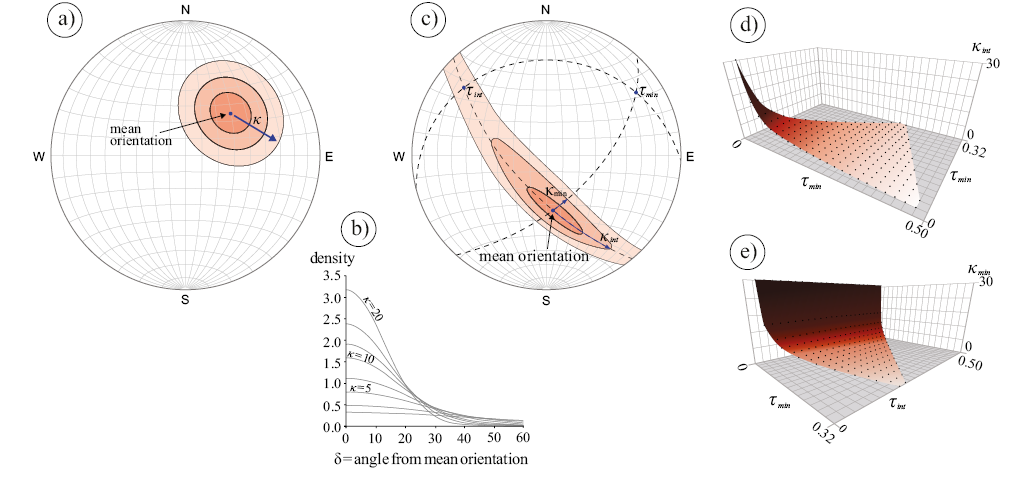
The first model, proposed by Fisher (Fisher, 1953), focuses on the distribution of poles symmetrically distributed around a mean vector (Figure 1a). The model conceptualizes a concept called Fisher’s spherical Probability Distribution Element (PDE), which provides the probability of finding a given direction within a unitary area element (dA), (Table 1). The model also considers a parameter known as Fisher’s κ (kappa), which increases as the concentration of poles around the mean orientation increases (Figure 1b).

The second model, proposed by Bingham (Bingham, 1964), focuses on the populations of data forming elongated clusters in the form of girdles. The model defines a confidence cone about the mean orientation, which intersection with the semi-sphere of the stratigraphic projection tends to form an ellipse (Figure 1c). The distorted region controlled the concentration parameters κint and κmin, they are intermediate and minimum concentration respectively and both are function of the normalized eigenvalues of the orientation’s tensor τ2 and τ3 (Figure 1d and 1e). Bingham’s spherical PDE is defined in Table 1.

 

METHODS

Methodology proposed

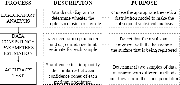
We propose a methodology to validate dip and dip direction data obtained from photogrammetry-derived point clouds. Such methodology is presented in Figure 2 and described in the following paragraphs. The methodology consists of three tests: the first two tests (“exploratory analysis” and “data consistency parameters estimation”) perform a quality check on the data, while the third test (“accuracy test”) compares the dip and dip direction data from photogrammetry against control measurements gathered using instruments such as a geological compass.

 

Exploratory analysis

This test aims at graphically identifying the distribution model that better fits the data and thence calculate the dispersion parameters. For this test, the pole distribution is plotted on an equal-area stereographic projection. The following step is realize a shape analysis using a Woodcock’s diagram (Woodcock, 1977).

Woodcock (1977) proposes representing each observation in terms of its direction cosines li, mi and ni. The set of all data’s directions can be represented as a 3 by 3 orientation matrix, T (Equation 1), by using xi, yi and zi, which are individual observation’s components without normalization in the X, Y and Z directions (Fernández, 2005) (1).

(1)

Considering that T is a symmetrical matrix, its eigenvalues, λ1, λ2, λ3, and its eigenvectors (ν1, ν2, ν3) can be calculated. The eigenvector ν1 corresponds to the direction of the smallest inertial moment, and thus, corresponds to the orientation with maximum density of observations. Meanwhile, the eigenvector ν3 corresponds to the largest inertial moment and corresponds to orientation with minimum observations’ density (Woodcock, 1977; Fernández, 2005). Expectedly, ν2 is perpendicular to eigenvectors ν1 and ν3.

The sum of the eigenvalues λ1, λ2 and λ3 equal the number of observations of the analyzed set (N), Equation 2 (Woodcock, 1977):

λ1 + λ2 + λ3 = N (2)

after normalization, we obtain that:

τ1 + τ2 + τ3 = 1 (3)

where: τ1 = λ1/N

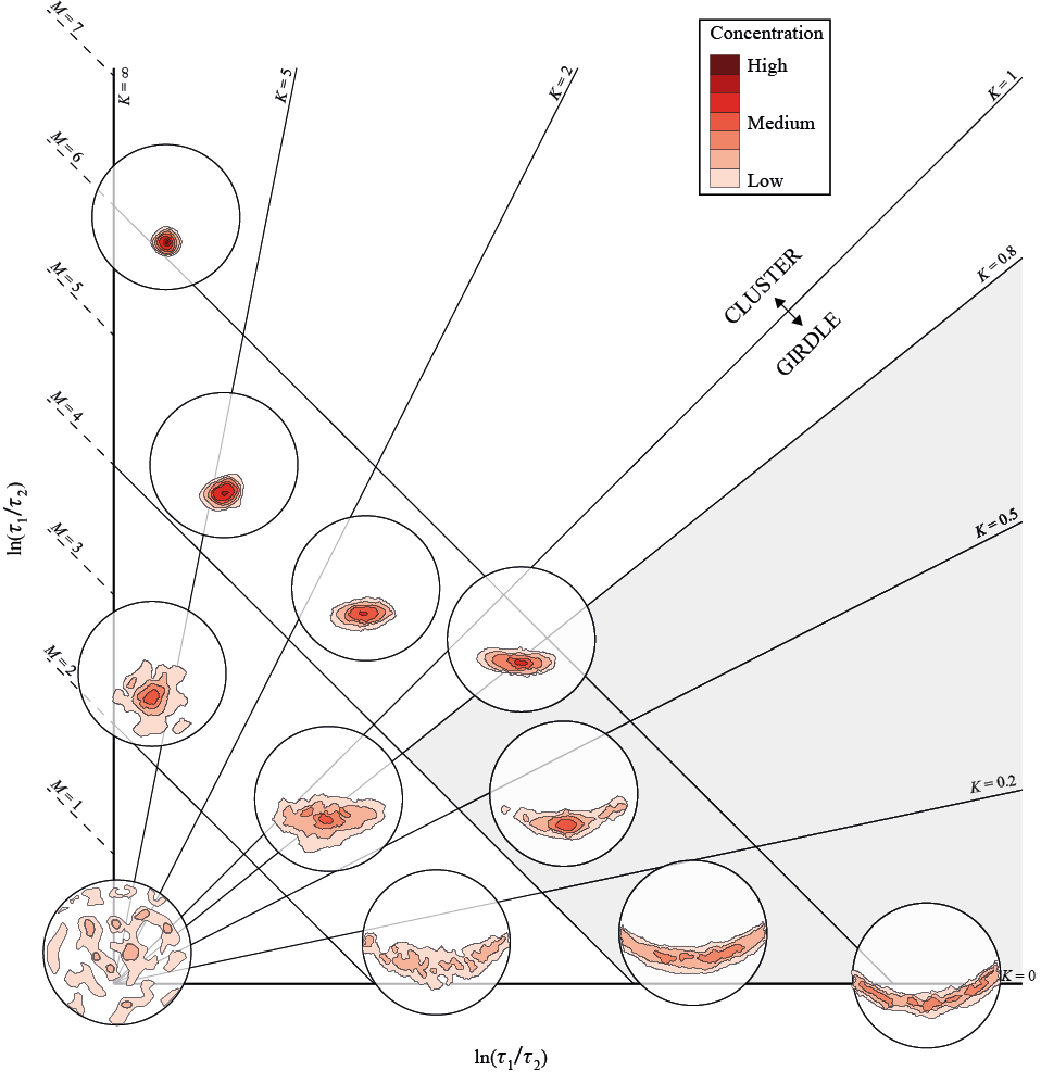
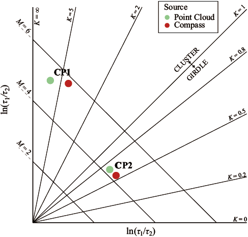
The normalized eigenvalues are ingested into a plot whose coordinate system has the comparison between τ1 and τ2 in the vertical axis and the comparison between τ2 and τ3 in the horizontal axis, forming Woodcock’s diagram (Figure 3). On the one hand, the degree of fit to a plane is indicated by the parameter M (Equation 4). The larger the M, the more coplanar the poles, regardless of their symmetry around a point (girdle) or around an axis (cluster).

(4)

On the other hand, the degree of collinearity is related with the parameter K (Equation 5). When K equals to 1, there’s not a clear criterium to define a cluster or a gridle. When 1, the data set falls into the classification of a girdle, and when ∞, the data set falls into the classification of a cluster.

(5)

Classic works on the treatment of paleomagnetic data (Tarling, 1983; McElhinny and McFadden, 2000; Tauxe, 2003; Butler, 2004) use the eigenvalues obtained from the direction matrix of the point cloud to be analyzed and plot them in Woodcoks diagram to obtain the model that better fits the data (cluster or girdle) (Woodcock, 1977). Thereafter, the best probabilistic approach is adopted, i.e. Fisher’s for clusters and Bingham’s for girdles. In this work, we propose adopting the same approach but for discontinuities’ orientation data.

(13)

(14)

Where I0 and I1 are modified Bessel’s functions of the first kind and orders zero and one respectively, τ2 and τ3 are derived from Equations 2 and 3, and θ is the cone angle. Mardia y Zemroch (1977) provide a table with the solutions to Equations 13 and 14 (Table 2) for values of κmin < 0.05. If necessary, for small values of τ2 and τ3, Equation 15 provides an acceptable approximation.

(15)

Finally, from the concentration values κmin and κint we can obtain the precision of the orientations in the minimum and intermediate direction (Borradaile, 2003) (Equations 16 and 17).

(16)

(17)

 

 

Figure 3. Woodcock’s diagram showing the cluster’s (circularly symmetric) and gridle’s (axially symmetric) fields. (Modified from Woodcock, 1997). Observe that the definition of Cluster or Girdle depends on the coordinate of the data points with respect to line K=1. Where K = ln(τ1/τ2)/ln(τ2/τ3) , and M = ln(τ1/τ3).

 

Table 2. Concentration parameters, κmin and κint for the Bingham (Mardia and Zemroch, 1977).

τ3 τ2	0.02	0.04	0.06	0.08	0.10	0.12	0.14	0.16	0.18	0.20	0.22	0.24	0.26	0.28	0.30	0.32
0.02	25.55
	25.55
0.04	25.56	13.11
	13.09	13.11
0.06	25.58	13.14	9.04
	9.00	9.02	9.04
0.08	25.60	13.16	9.07	7.04
	6.98	7.00	7.02	7.04
0.10	25.62	13.18	9.08	7.04	5.80
	5.76	5.78	5.79	5.80	5.80										κint	25.61
0.12	25.63	13.19	9.09	7.04	5.79	4.92									κmin	2.43
	4.92	4.93	4.94	4.94	4.93	4.92
0.14	25.64	13.20	9.09	7.03	5.77	4.90	4.23
	4.30	4.30	4.30	4.29	4.28	4.26	4.23
0.16	25.65	13.20	9.08	7.02	5.75	4.87	4.20	3.66
	3.80	3.80	3.79	3.78	3.76	3.73	3.70	3.66
0.18	25.65	13.19	9.07	7.00	5.73	4.84	4.16	3.62	3.16
	3.38	3.38	3.36	3.35	3.32	3.29	3.25	3.21	3.16
0.20	25.64	13.18	9.05	6.97	5.69	4.80	4.13	3.57	3.11	2.71
	3.03	3.01	3.00	2.97	2.94	2.91	2.86	2.82	2.77	2.71
0.22	25.63	13.17	9.03	6.94	5.66	4.76	4.07	3.52	3.05	2.65	2.29
	2.71	2.70	2.67	2.64	2.61	2.57	2.52	2.47	2.41	2.35	2.29
0.24	25.61	13.14	9.00	6.91	5.62	4.71	4.02	3.46	2.99	2.58	2.22	1.89
	2.43	2.41	2.38	2.35	2.31	2.26	2.21	2.16	2.10	2.03	1.96	1.89
0.26	25.59	13.12	8.97	6.87	5.57	4.66	3.97	3.40	2.93	2.52	2.15	1.81	1.50
	2.18	2.15	2.12	2.08	2.03	1.98	1.93	1.87	1.81	1.74	1.66	1.58	1.50
0.28	25.57	13.09	8.93	6.83	5.52	4.61	3.91	3.34	2.86	2.44	2.07	1.72	1.41	1.11
	1.94	1.91	1.87	1.83	1.78	1.73	1.67	1.60	1.53	1.46	1.38	1.29	1.20	1.11
0.30	25.54	13.05	8.89	6.78	5.47	4.55	3.84	3.27	2.79	2.36	1.98	1.63	1.31	1.00	0.71
	1.72	1.68	1.64	1.59	1.54	1.48	1.42	1.35	1.27	1.20	1.11	1.02	0.92	0.82	0.71
0.32	25.50	13.01	8.84	6.73	5.41	4.48	3.77	3.20	2.71	2.28	1.89	1.54	1.21	0.89	0.59	0.29
	1.51	1.47	1.42	1.37	1.31	1.25	1.18	1.11	1.03	0.94	0.85	0.76	0.65	0.54	0.42	0.29
0.34	25.46	12.96	8.79	6.67	5.35	4.42	3.70	3.12	2.62	2.19	1.79	1.43	1.09	0.77	0.46	0.15
	1.31	1.27	1.22	1.16	1.14	1.03	0.96	0.88	0.79	0.70	0.60	0.50	0.39	0.27	0.14	0.00
0.36	25.42	12.91	8.73	6.61	5.28	4.34	3.62	3.03	2.53	2.09	1.69	1.32	0.97	0.64
	1.12	1.07	1.02	0.96	0.89	0.81	0.74	0.65	0.56	0.46	0.36	0.25	0.13	0.00
0.38	25.37	12.86	8.67	6.54	5.21	4.26	3.35	2.94	2.43	1.99	1.58	1.20
	0.94	0.89	0.82	0.76	0.68	0.61	0.52	0.43	0.34	0.23	0.12	0.00
0.40	25.31	12.80	8.60	6.47	5.13	4.18	3.45	2.85	2.33	1.87
	0.76	0.70	0.64	0.56	0.49	0.40	0.31	0.22	0.11	0.00
0.42	25.25	12.73	8.53	6.39	5.05	4.09	3.35	2.74
	0.59	0.52	0.45	0.37	0.29	0.20	0.10	0.00
0.44	25.19	12.66	8.45	6.31	4.96	3.99
	0.42	0.35	0.27	0.19	0.10	0.00
0.46	25.12	12.58	8.37	6.22
	0.25	0.17	0.09	0.00
0.48	25.04	12.50
	0.08	0.00

Figure 4. “La Escuelita” rock outcrop wall (19.3341°, -99.1933°). (a) Panoramic view, yellow polyline indicates a discontinuity surface between two lava flows and red polygons show the location Control Polygons 1 and 2. (b) Red meshes show the discretization, of CP1 corresponds to a planar discontinuity surface, while CP2 corresponds to a curved one. (c) Roughness detail for one element on the mesh. (d) Show a section of planar surface (CP1) and curved surface (CP2).

Table 3. Eigenvalues and logarithm of eigenvalues ratios for CP1 and CP2.

Eigenvalues	CP1			CP2
	Compass	Point Cloud		Compass	Point cloud
τ1	0.9848	0.9839		0.8079	0.8316
τ2	0.0114	0.0102		0.1793	0.1557
τ3	0.0037	0.0059		0.0128	0.0127
ln(τ1/τ2)	4.459	4.569		1.5054	1.6754
ln(τ2/τ3)	1.125	0.547		2.6396	2.5063

 

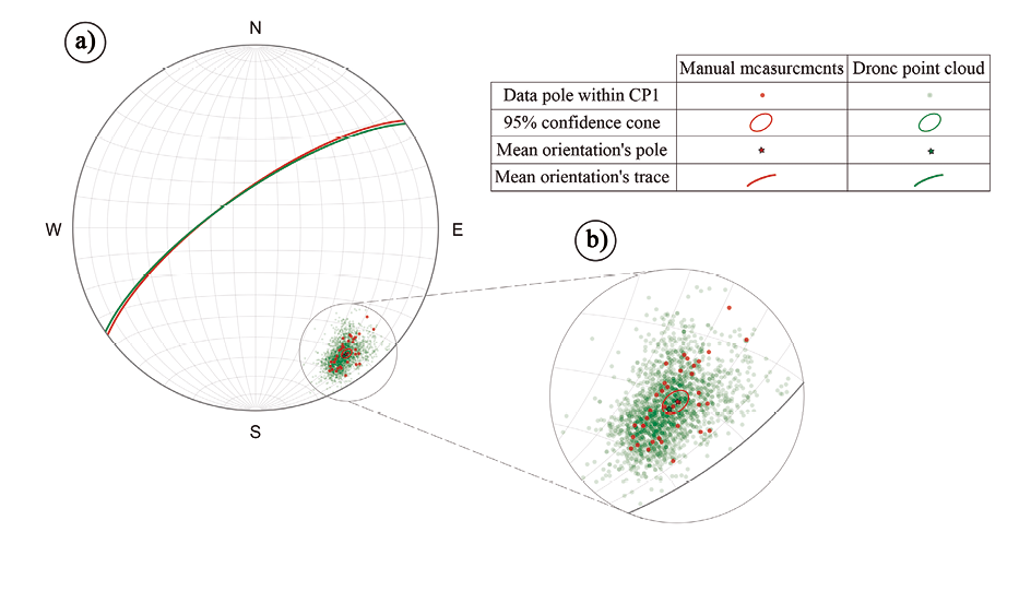
Figure 6. (a) Stereographical representation of CP1 data and (b) the confidence cones detail obtained using Fisher’s model

 

Table 4. Results summary of the dispersion parameters and accuracy test estimations for CP1 with Fisher’s model.

CP1	Manual measurements		Point cloud
Mean orientation (Dip, Dip direction)	73.76°, 324.08°		74.03°, 325.31°
N	36		2036
R	35.72		2019.48
κ	127.39		123.17
α95	2.07°		0.28°
Accuracy test
Angular deviation	1.21
F-test (95 %)	0.97 <3

 

DISCUSION

The analysis of CP1 from Fisher’s model revealed high κ values (Table 4), both for the compass data (κ = 127.4) and for the point cloud data (κ = 123.2), which indicates that the mean direction obtained for each case is representative of that sample. Studies from Jordá Bordehore et al. (2017) and Drews et al. (2018) showed cases where the condition of κ is also greater than 10, from 54 to 166 for the first and between 61 and 220 for the second (Table 7), which is consistent with our results. These studies also show that κ values can vary remarkably between orientation data obtained with a compass and point clouds for the same discontinuity surface (Table 7), indicating greater or lesser concentration but identifying a mean orientation, which is not the case of our results.

However, α95 values in our study differ by almost 2° between the manual and the point cloud measurements α95 (manual) = 2.07° and α95 (point cloud) = 0.28°, which means that the value of the mean orientation from the point cloud is of greater confidence. This contrast is observed when comparing the confidence cones’ size in Figure 6b and is partly due to the large amount of data from the point cloud to capture the flat surface CP1.

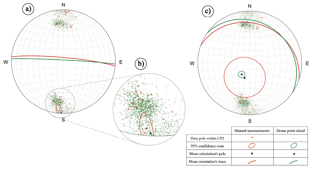
For CP2, we used Bingham model. The values of κmin and κint are almost identical for manual measurement, and the values of α95(min) is 3.58 and α95(int) is 3.6. These values define opened confidence cones compared to the results from the point cloud measurements, where are α95(min) point cloud is 0.47 and α95(int) point cloud is 1.52.

In contrast, point cloud measurements describe κmin>κint (Table 5), as expected according to Mardia and Zemroch (1977), since the sample clusters more in the minimum direction (see Figure 7b). As κint<10, the data is scattered in that direction, but considering κmin>1, we can say that the sample has a preferential orientation. The value of α95 of greatest interest is α95(min) since the confidence cone will be smaller in this direction.

As can be seen in Table 5 and Figure 7a, α95(min) manual = 13.6° and α95(min) point cloud = 1.52°, which indicates, as in the previous case, that the measurements obtained for the mean orientation from the point cloud represent the complexity of the CP2 surface more reliably than manual measurements. This reliability is partly associated with the large number of measurements available from the point cloud compared to those of the manual measurements, 2000 vs. 36 measurements respectively.

The hypothesis tests (based on F-test) for CP1 and CP2 were successful, considering that the control data were manual, and that the confidence cone generated from the point cloud remains within the cone from the manual data. (Figures 6a and 7a). Consequently, we accepted the null hypothesis that the two measurements represent the same discontinuity for both cases (Tables 4 and 5).

At this point, it is essential to note that other works commonly adopt Fisher’s model (i.e., Table 6), as it is a common practice in geotechnical engineering to simplify surfaces as planes (Jordá Bordehore et al., 2017; Drews et al., 2018). However, and for the sake of argument, let us analyze the results CP2 using Fisher’s model (Table 8, Figure 7c). Consider that if we treat CP2 as a plane, the data obtained would indicate that the sample is very dispersed, and therefore there would not be a clear mean orientation (Table 6).

This observation becomes more tangible in the manual measurements, where κ = 1.76, clearly below the recommended value of 10, also α95 (manual) = 32° is a very high value that defines a large confidence cone. Although the point cloud’s confidence cone is within the cone from the manual data (from an informal point of view), this cone’s value is much higher than that of tables when performing the F-test. That is why we discard the hypothesis that both samples belong to the same discontinuity.

One of our methodology’s applications is to validate discontinuity surfaces from point clouds obtained with remote sensing tools using steps 1 and 2. Additionally, if control measurements are available, step 3 helps us calibrate and compare the data objectively and quantitatively.

In addition, in applications such as the measurement and classification of folds like Ramsay’s classification (Ramsay and Huber 1987) and slope stability analysis, it can help to carry out studies with a high resolution by taking advantage of the number of measurements from point clouds obtained with a remote sensing tool, thus avoiding simplification when the conditions for manual data collection are complicated.

For example, a common simplification in rock slope stability analysis assumes that all discontinuities families are plane surfaces (Hoek and Bray, 1981; Goodman, 1989; Hudson and Harrison, 1997; Kliche, 1999). The simplification in our CP2 example would be to analyze the curved plane as two families, one with the dip towards the north and the other towards the south (Figure 7). However, the curvature of the surface would be neglected, which in practical terms could mean an increase or a reduction in the Safety Factor using a limit equilibrium stability analysis.

Most of the algorithms reported in the literature base the semi-automatic identification of discontinuity families from point clouds on the detection of planes only gm, which in general simplifies and solves the geometry almost realistically. However, in some geological environments such as curved fractures by cooling (Pollard and Aydin, 1988; Glastonbury and Fell, 2000; Sainsbury and Sainsbury 2013; Stead et al., 2006; Crider, 2015; Stead and Wolter, 2015), discontinuities outline curved surfaces that require the intervention of the Bingham model, which can be analyzed with the methodology here proposed.

Although our experiment was controlled and automatically identified surfaces were not tested with other available algorithms, this methodology could be used when applying algorithms that identify curved surfaces such as those of Schnabel et al. (2007) or Liu et al. (2019). In this sense, this methodology is not restricted to Rock Mechanics applications, but it can be applied in Structural Geology for the validation in the measurement and classification of geological folds. Besides, in those cases where the condition of discontinuity surfaces is measured and is necessary to validate the quality of the data obtained from a point cloud.

 

 

 

CONCLUSIONS

In this work, a methodology is proposed to validate the quality of directional data such as point clouds or data acquired manually using a geological compass (contingent on sufficient data). The proposed methodology consists of three steps which are based on spherical statistics.

The first step is an exploratory analysis of shape to define which statistics distribution model to use. If the distribution of the data is circularly symmetric, the model to be used will be Fisher’s and when the symmetry is axial in the data, then it is proposed to use the Bingham model. The second step is to calculate the consistency parameters of the data, that is, the concentration parameter (κ) and confidence cone (α95). These parameters indicate how dispersed the sample is and the reliability of finding the mean orientation with a confidence limit of 95 %. The third step is a hypothesis test to determine if two groups of data represent the same surface in the mass rock.

We verify that the methodology allows obtaining parameters that validate the quality of the directional data and is easy to apply. Although the common professional practice is to treat discontinuities as planar surfaces to apply Fisher’s model, we observed that there are surfaces that may resemble planes but statistically behave like non-planar surfaces which can be better represented using Bingham’s model. The tendency to non-planarity is often considered as roughness and accounted for using parameters such as the Joint Roughness Coefficient (JRC) (Barton, 1973). However, such parameter works at a scale which usually does not impact the geometry used in a kinematic analysis of slope stability. Therefore, the choice of using either Fisher or Bingham’s model becomes very important.

The limitations of the drone-assisted dataset used in this work includes the illumination of the observed discontinuities, in terms of the need to have a free face and must be free of vegetation. However, our dataset did allow us to map nonplanar discontinuities, which would be difficult to identify in a normal field survey without doing systematic measurements for 0.60 by 0.60 m polygons as done in this work.

 

SUPPLEMENTARY MATERIAL

The Table S1 "Distribution F-Fisher values" can be found at <www.rmcg.unam.mx>, in the abstract-preview page of this paper.

 

ACKNOWLEDGEMENTS

This research has been financed with the UNAM-PAPIIT Group IV100117 project, carried out between the Centro de Geociencias and the Facultad de Ingeniería (by Luca Ferrari), both institutions of the Universidad Nacional Autónoma de México.

We would also like to thank the Editor-in-chief (Dr. Angel Francisco Nieto Samaniego) and Reviewers (Dr. Alberto Vázquez Serrano and other anonymous reviewer) for providing us observations and recommendations based on the constructive reviews of our manuscript.

 

REFERENCES

AgisoftPhotoScan Professional, version 1.5, Educational license, (Software), 2019, Retrieved from http://www.agisoft.com/downloads/installer/

Allmendinger, R.W., Cardozo N., Fisher D.M. 2011, Structural geology algorithms: Vectors and tensors: Cambridge, UK, Cambridge University Press, 289 pp

Badilla, C.R.R., 1977, EstudioPetrológico de la Lava de la ParteNoreste del Pedregal de San Ángel, D.F.:Boletín de la Sociedad Geológica Mexicana, XXXVIII (1), 40-57, doi: 10.18268/BSGM1977v38n1a4

Barton, N., 1973, Review of a new shear-strength criterion for rock joints: Engineering Geology, 7(4),287-332, doi: 10.1016/0013-7952(73)90013-6

Bingham, C., 1964, Distributions on the sphere and on the projective plane. New Haven, U.S.A, Yale University, PhD Thesis, 136 pp.

Borradaile, G., 2003, Statistics of Earth Science Data, Their Distribution in Time, Space, and Orientation:Berlin, Heidelberg, Springer, 353 pp.

Borrmann, D., Elseberg, J., Lingemann, K., Núchter, A., 2011, The 3D Hough Transform for plane detection in point clouds: A review and a new accumulator design: 3D Research, 3, 1-13, doi: 10.1007/3DRes.02(2011)3

Butler, R.F., 2004, Paleomagnetism: magnetic domains to geologic terranes, Paleomagnetism: Magnetic Domains to Geologic Terranes: Portland, OR, Blackwell Scientific Publications, 336 pp.

Buyer, A., Aichinger, S., Schubert, W., 2020, Applying photogrammetry and semi-automated joint mapping for rock mass characterization: Engineering Geology, 264, doi:10.1016/j.enggeo.2019.105332

Cloud Compare, version 2.11, 2019, Daniel G.M., Retrieved from http://www.cloudcompare.org/, (Software). February, 2002.

Crider, J., 2015, The initiation of brittle faults in crystalline rock:Journal of Structural Geology, 77, 159-174, doi: 10.1016/j.jsg.2015.05.001

Davis, J.C., 2002, Statistics and Data Analysis in Geology: New York, USA, Wiley, 656 pp.

Davis, G.H., Reynolds, S.J., Kluth, C., 2011, Structural geology of rocks and regions: New York, USA, Wiley, 864 pp.

Delgado, H., Molinero, R., Cervantes, P., Nieto-Obregon, J., Lozano-Santa Cruz R., Macías-González, H. L., Medoza-Rosales, C., Silva-Romo, G., 1998, Geology of Xitle Volcano in Southern Mexico City -a 2000 year- old monogenetic volcano in an urban area: Revista Mexicana de Ciencias Geológicas, 15(2), 115-131.

Drews, T., Miernik, G., Anders, K., Höfle, B., Profe, J., Emmerich, A., Bechstädt, T., 2018, Validation of fracture data recognition in rock masses by automated plane detection in 3D point clouds: International Journal of Rock Mechanics and Mining Sciences, 109, 19-31. doi: 10.1016/j.ijrmms.2018.06.023

Fernández, O., 2005, Obtaining a best fitting plane through 3D georeferenced data: Journal of Structural Geology, 27(5), 855-858, doi: 10.1016/j.jsg.2004.12.004

Fetter, C.W., 2001, Applied hydrogeology: New York, USA, Macmillan College Publishing Company, 58 pp.

Fisher, R., 1953, Dispersion on a Sphere, Proceedings of the Royal Society of London Series A: Mathematical, Physical and Engineering Sciences, 217(1130), 295-305. doi: 10.1098/rspa.1953.0064

Fisher, N.I., Lewis, T., Embleton, B.J.J., 1987, Statistical analysis of spherical data: Cambridge, UK, Cambridge University Press, doi: 10.1017/CBO9780511623059

Glastonbury, J., Fell, R., 2000, Report on the analysis of "rapid" natural rock slope failures: New South Wales, Australia, University of New South Wales, School of Civil and Environmental Enginnering Report No. R390.

Goodman, R.E., 1989, Introduction to Rock Mechanics: New York, USA, Wiley, 576 pp.

Hoek, E. and Bray J., 1981, Rock Slope Engineering: London, UK, Insitution of Mining and Metallurgy by Taylor and Francis, 357 pp.

Hudson, A.J., Harrison, P.J., 1997, Engineering Rock Mechanics, An Introduction to the principles: Amsterdam, NED. Elsevier Science, 456 pp.

Jordá Bordehore, L., Riquelme, A., Cano, M., Tomas, R., 2017, Comparing manual and remote sensing field discontinuity collection used in kinematic stability assessment of failed rock slopes: International Journal of Rock Mechanics and Mining Sciences. 97, 24-32. doi: 10.1016/j.ijrmms.2017.06.004

Kliche, C.A., 1999, Rock Slope Stability: Littleton, CO, Society for Mining, Metallurgy, and Exploration,253 pp.

Leng X., Xiao, J., Wang Y., 2016, A multi-scale plane-detection method based on the Hough transform and region growing: The Photogrametric Record, 31(154), 166-192, doi: 10.1111/phor.12145

Lerche, I., 1997, Geological Risk and Uncertainty in Oil Exploration: San Diego, USA, Academic Pr, 658 pp.

Li, X., Chen, Z., Chen, J., Zhu, H., 2019, Automatic characterization of rock mass discontinuities using 3D point clouds: Engineering Geology 259, doi:10.1016/j.enggeo.2019.05.008

Liu, L., Xiao, J., Wang, Y., 2019, Major Orientation Estimation-Based Rock Surface Extraction for 3D Rock-Mass Point Clouds: Remote Sensing, 11(6), 1-24, doi: 10.3390/rs11060635

Mancera-Alejándrez, J., Villarreal-Rubio, E., Macías-Medrano, S., Hernández-Espriu, A., López-Molina, 2020, Statistical validation of dip and dip direction of discontinuity planes of rock masses obtained from point clouds acquired with drone, in Rock Mechanics for Natural Resources and Infrastructure Development:Foz do Iguaçu; Brazil, Proceedings of the 14th International Congress on Rock Mechanics and Rock Engineering, ISRM 2019, 2171-2178, ISBN 978-0-367-42284-4.

Mardia, K.V., 1972, Statistics of Directional Data: Orlando, Florida, USA, Academic Press, Inc., 357 pp.

Mardia, K.V., Zemroch, P.J., 1977, Table of maximum likelihood estimates for the bingham distribution: Journal of Statistical Computation and Simulation, 6, 29-34. doi: 10.1080/00949657708810165

Marshak, S., Mitra, G., 1988, Basic Methods of Structural Geology, Prentice Hall Englewood, New Jersey, 446 pp.

McFadden, M., McFadden, P., 2000, Paleomagnetism, Continents and Oceans: San Diego, USA, Academic Press., 386 pp.

Priest, S.D., 1993, Discontinuity Analysis For Rock Engineering: London, UK, Chapman and Hall, 473 pp.

Pollard, D.D., Aydin A., 1988, Progress in understanding jointing over the past century: Geological Society of America Bulletin, 100(8), 1181-1204, doi: 10.1130/0016-7606(1988)100<1181:PIUJOT>2.3.CO;2

Ramsay J.G., Huber M.I., 1987, The Techniques of Modern Structural Geology, Volume 2: Folds and Fractures: London , Pergamon Press, 391 pp.

Riquelme, A.J., Abellán, A., Tomás, R., Jaboyedoff, M., 2014, A new approach for semiautomatic rock mass joints recognition from 3D point clouds: Computer and Geosciences, 68, 38-52, doi:10.1016/j.cageo.2014.03.014.

Rusu, R.B., Cousins, S., 2011, 3D is here:Point Cloud Library (PCL), in IEEE International Conference on Robotics and Automation: CA USA, Institute of Electrical and Electronics Engineers (IEEE), 1-4, doi: 10.1109/ICRA.2011.598056

Sainsbury, DP and Sainsbury, B 2013, ‘Three-dimensional analysis of pit slope stability in anisotropic rock masses’, in PM Dight (ed.), Slope Stability 2013: Proceedings of the 2013 International Symposium on Slope Stability in Open Pit Mining and Civil Engineering, Australian Centre for Geomechanics, Perth, 683-695, https://doi.org/10.36487/ACG_rep/1308_45_Sainsbury

Schmiter, V.E., 1953, Investigación petrológica en las lavas del Pedregal de San Ángel, in Memorias del Congreso Científico Mexicano, Ciencias físicas y Matemáticas: Mexico City, Mexico, Universidad Nacional Autónoma de México, 218-237.

Schnabel, R., Wahl, R., Klein, R., 2007, Efficient RANSAC for Point-Cloud Shape Detection: Computer Graphics Forum, 26(2), 214-226.

Siebe, C., 2008, La erupción del volcán Xitle y las lavas del Pedregal hace 1670± 35 años AP y sus implicaciones, in Biodiversidad del ecosistema del Pedregal de San Angel, Mexico City, Mexico, Universidad Nacional Autónoma de México, 43-49.

Stead, D., Eberhardt, E., Coggan, J.S., 2006, Developments in the characterization of complex rock slope deformation and failure using numerical modelling techniques: Engineering Geology, 83(1-3), 217-235, doi:10.1016/j.enggeo.2005.06.033

Stead, D., Wolter, A., 2015, A critical review of rock slope failure mechanisms: The importance of structural geology: Journal of structural Geology, 74, 1-23, doi: 10.1016/j.jsg.2015.02.002

Sturzenegger, M., Stead, D., 2009, Close-range terrestrial digital photogrammetry and terrestrial laser scanning for discontinuity characterization on rock cuts: Engineering Geology,106(3-4), 163-182. doi: 10.1016/j.enggeo.2009.03.004

Tarling, D.H., 1983, Palaeomagnetism: Principles and Aplications in Geology, Geophysics and Archaeology: New York, USA, Chapman and Hall, 380 pp.

Tauxe, L., 2003, Paleomagnetic Principles and Practice. Kluwer Academic Publishers (Modern Approaches in Geophysics): Dordrecht, Netherlands, Kluber Academic Publishers, 301 pp.

Watson, G.S., 1965, Equatorial Distributions on a Sphere: Biometrika, 52(1), 193-201. doi: 10.2307/2333824

Woodcock, N.H., 1977, Specification of fabric shapes using an eigenvalue method: Geological Society of America Bulletin, 88(9), 1231-1236, doi: 10.1130/001-7606(1977)88<1231:SOFSUA>2.0.CO;2